Titanic - Machine Learning from Disaster
The sinking of the Titanic is one of the most infamous shipwrecks in history. On April 15, 1912, during her maiden voyage, the widely considered “unsinkable” RMS Titanic sank after colliding with an iceberg. Unfortunately, there weren’t enough lifeboats for everyone onboard, resulting in the death of 1502 out of 2224 passengers and crew. While there was some element of luck involved in surviving, it seems some groups of people were more likely to survive than others.
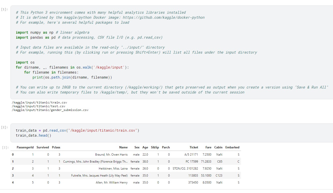
We will make use of two similar datasets that include passenger information like name, age, gender, socio-economic class, etc. One dataset is titled train.csv and the other is titled test.csv. Train.csv will contain the details of a subset of the passengers on board (891 to be exact) and importantly, will reveal whether they survived or not, also known as the “ground truth”. The test.csv dataset contains similar information but does not disclose the “ground truth” for each passenger. We will predict these outcomes.
Explanation
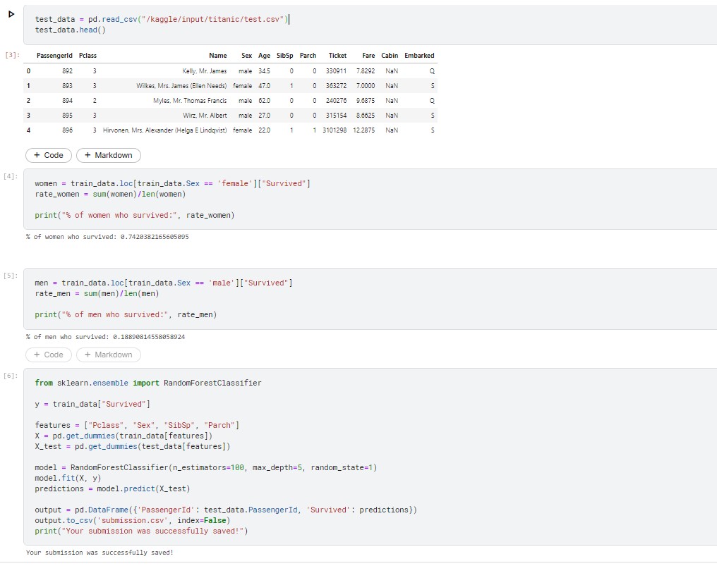
The above code demonstrates the calculation of survival percentages for male and female passengers. It is evident that the survival rate for women was significantly higher, with nearly 75% of them surviving, while only 19% of men survived. This indicates that gender is a crucial factor in determining survival, and the gender_submission.csv file can serve as a decent initial estimate.
However, it is important to note that this submission is based solely on one column, and more complex patterns can be discovered by considering multiple columns, which could potentially lead to more accurate predictions. Nevertheless, analyzing multiple columns simultaneously can be a challenging and time-consuming task. This is where machine learning comes into play, allowing us to automate the process of pattern recognition and analysis.
We will create a random forest model, which comprises several "trees." Each tree will examine the data of every passenger individually and decide whether the individual survived or not. The random forest model then combines the votes of each tree to make a democratic decision, with the outcome receiving the most votes considered as the final prediction.The code in the cell seeks out patterns in four different columns ("Pclass", "Sex", "SibSp", and "Parch") of the data. It uses these patterns in the train.csv file to construct the trees in the random forest model. The model then uses these trees to generate predictions for the passengers in test.csv. Finally, the new predictions are saved as a CSV file called submission.csv.
Contribution
Here the training dataset is analyzed for any null values in the individual columns. The columns 'Age' and 'Embarked' has null values in it, so we will try to fix the issue by replacing null values with the appropriate mean or mode values of that attribute data. Now we will drop the irrelevant features that does not help in analyzing the Disaster, by doing this we can prevent overfitting.
train_data.isnull().any()
train_data['Age'].fillna((train_data['Age'].mean()),inplace=True)
train_data=train_data.drop(['Embarked','Cabin','Fare','Ticket','Name'],axis=1)
test_data['Age'].fillna((test_data['Age'].mean()),inplace=True)
test_data=test_data.drop(['Embarked','Cabin','Fare','Ticket','Name'],axis=1)
Feature engineering is a machine learning technique that leverages data to create new variables that aren’t in the training set. Here we have created 'FamilyGroup' column by adding the number of siblings and number of parents data which represents the total number of family members that each passenger has boarded the ship. Similarly I have created a column 'AgeGroup' by dividing the age data into four groups
train_data["FamilyGroup"] = train_data["SibSp"] + train_data["Parch"]
test_data["FamilyGroup"] = test_data["SibSp"] + test_data["Parch"]
train_data["AgeGroup"] = pd.cut(train_data["Age"], bins=[0, 18, 35, 50, 100], labels=["Child", "Adult1", "Adult2", "Elderly"])
test_data["AgeGroup"] = pd.cut(test_data["Age"], bins=[0, 18, 35, 50, 100], labels=["Child", "Adult1", "Adult2", "Elderly"])
Feature extraction is the process of extracting features from a data set to identify useful information. Without distorting the original relationships or significant information, this compresses the amount of data into manageable quantities for algorithms to process. Here we have taken the columns "Pclass", "Sex", "FamilyGroup" and "AgeGroup" as features.
features = ["Pclass", "Sex", "FamilyGroup", "AgeGroup"]
X = pd.get_dummies(train_data[features])
y = train_data["Survived"]
X_test = pd.get_dummies(test_data[features])
After creating an instance of the RandomForestClassifier class, we can use the fit method to train the model on a set of input features and their corresponding labels. Once the training is complete, the model can then be used to make predictions on new data that it has not seen before using the predict method.
# Tune Model Hyperparameters
from sklearn.model_selection import GridSearchCV
from sklearn.ensemble import RandomForestClassifier
param_grid = {
"n_estimators": [50, 100, 150],
"max_depth": [3, 5, 7],
"min_samples_split": [2, 5, 10]
}
rf = RandomForestClassifier(random_state=1)
grid_search = GridSearchCV(rf, param_grid=param_grid, cv=5)
grid_search.fit(X, y)
best_rf = grid_search.best_estimator_
The below code performs 5-fold cross-validation on the machine learning model using mean imputation strategy.
X = X.fillna(X.mean())
X_test = X_test.fillna(X_test.mean())
# Perform Cross-validation
from sklearn.model_selection import cross_val_score
cv_scores = cross_val_score(model, X, y, cv=5)
print("Cross-validation scores:", cv_scores)
print("Mean cross-validation score:", cv_scores.mean())
The below code trains the model using the input data X and the target variable y. It then makes predictions on the test data X_test using the trained model, and saves the predictions to a CSV file.
best_rf.fit(X, y)
predictions = best_rf.predict(X_test)
predictions = model.predict(X_test)
output = pd.DataFrame({'PassengerId': test_data.PassengerId, 'Survived': predictions})
output.to_csv('submission2.csv', index=False)
Original Score versus Improved Score

